Maxwell–Boltzmann distribution
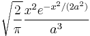
| Probability density function |
|
| Cumulative distribution function |
|
| Parameters |  |
|---|---|
| Support |  |
 |
|
| CDF | 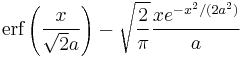 where erf is the Error function where erf is the Error function |
| Mean |  |
| Mode |  |
| Variance | 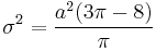 |
| Skewness | 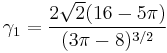 |
| Ex. kurtosis |  |
| Entropy |  |
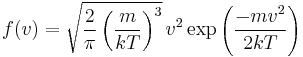
The Maxwell–Boltzmann distribution describes particle speeds in gases, where the particles do not constantly interact with each other but move freely between short collisions. It describes the probability of a particle's speed (the magnitude of its velocity vector) being near a given value as a function of the temperature of the system, the mass of the particle, and that speed value. This probability distribution is named after James Clerk Maxwell and Ludwig Boltzmann.
The Maxwell–Boltzmann distribution is usually thought of as the distribution for molecular speeds, but it can also refer to the distribution for velocities, momenta, and magnitude of the momenta of the molecules, each of which will have a different probability distribution function, all of which are related. Unless otherwise stated, this article will use "Maxwell–Boltzmann distribution" to refer to the distribution of speed. This distribution can be thought of as the magnitude of a 3-dimensional vector whose components are independent and normally distributed with mean 0 and standard deviation  . If
. If  are distributed as
  , then
is distributed as a Maxwell–Boltzmann distribution with parameter . Apart from the scale parameter , the distribution is identical to the chi distribution with 3 degrees of freedom.
Contents |
Physical applications of the Maxwell–Boltzmann distribution
The Maxwell–Boltzmann distribution applies to ideal gases close to thermodynamic equilibrium with negligible quantum effects and at non-relativistic speeds. It forms the basis of the kinetic theory of gases, which explains many fundamental gas properties, including pressure and diffusion.
Derivation
The original derivation by Maxwell assumed all three directions would behave in the same fashion, but a later derivation by Boltzmann dropped this assumption using kinetic theory. The Maxwell–Boltzmann distribution (for energies) can now most readily be derived from the Boltzmann distribution for energies (see also the Maxwell–Boltzmann statistics of statistical mechanics):
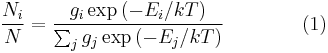
where:
- i is the microstate (indicating one configuration particle quantum states - see partition function).
- Ei is the energy level of microstate i.
- T is the equilibrium temperature of the system.
- gi is the degeneracy factor, or number of degenerate microstates which have the same energy level
- k is the Boltzmann constant.
- Ni is the number of molecules at equilibrium temperature T, in a state i which has energy Ei and degeneracy gi.
- N is the total number of molecules in the system.
Note that sometimes the above equation is written without the degeneracy factor gi. In this case the index i will specify an individual state, rather than a set of gi states having the same energy Ei. Because velocity and speed are related to energy, Equation 1 can be used to derive relationships between temperature and the speeds of molecules in a gas. The denominator in this equation is known as the canonical partition function.
Distribution for the momentum vector
What follows is a derivation wildly different from the derivation described by James Clerk Maxwell and later described with fewer assumptions by Ludwig Boltzmann. Instead it is close to Boltzmann's later approach of 1877.
For the case of an "ideal gas" consisting of non-interacting atoms in the ground state, all energy is in the form of kinetic energy, and gi is constant for all i. The relationship between kinetic energy and momentum for massive particles is
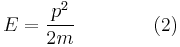
where p2 is the square of the momentum vector p = [px, py, pz]. We may therefore rewrite Equation 1 as:
![\frac{N_i}{N} =
\frac{1}{Z}
\exp \left[
-\frac{p_{i, x}^2 %2B p_{i, y}^2 %2B p_{i, z}^2}{2mkT}
\right]
\qquad\qquad (3)](/2012-wikipedia_en_all_nopic_01_2012/I/a3dfa5dc5d9cf628ca1713c51d76a57e.png)
where Z is the partition function, corresponding to the denominator in Equation 1. Here m is the molecular mass of the gas, T is the thermodynamic temperature and k is the Boltzmann constant. This distribution of Ni/N is proportional to the probability density function fp for finding a molecule with these values of momentum components, so:
![f_\mathbf{p} (p_x, p_y, p_z) =
\frac{c}{Z}
\exp \left[
-\frac{p_x^2 %2B p_y^2 %2B p_z^2}{2mkT}
\right].
\qquad\qquad (4)](/2012-wikipedia_en_all_nopic_01_2012/I/abb62eba6fbe952980c6fa4d5f57618c.png)
The normalizing constant c, can be determined by recognizing that the probability of a molecule having any momentum must be 1. Therefore the integral of equation 4 over all px, py, and pz must be 1.
It can be shown that:
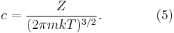
Substituting Equation 5 into Equation 4 gives:
![f_\mathbf{p} (p_x, p_y, p_z) =
\left( \frac{1}{2 \pi mkT} \right)^{3/2}
\exp \left[
-\frac{p_x^2 %2B p_y^2 %2B p_z^2}{2mkT}
\right].
\qquad\qquad (6)](/2012-wikipedia_en_all_nopic_01_2012/I/c719a3700cd88ff5886b1d1d002a0ba6.png)
The distribution is seen to be the product of three independent normally distributed variables  ,
,  , and
, and  , with variance
  . Additionally, it can be seen that the magnitude of momentum will be distributed as a Maxwell–Boltzmann distribution, with
  . The Maxwell–Boltzmann distribution for the momentum (or equally for the velocities) can be obtained more fundamentally using the H-theorem at equilibrium within the kinetic theory framework.
Distribution for the energy
Using p² = 2mE, and the distribution function for the magnitude of the momentum (see below), we get the energy distribution:
![f_E\,dE=f_p\left(\frac{dp}{dE}\right)\,dE =2\sqrt{\frac{E}{\pi}} \left(\frac{1}{kT} \right)^{3/2}\exp\left[\frac{-E}{kT}\right]\,dE. \qquad
\qquad(7)](/2012-wikipedia_en_all_nopic_01_2012/I/e13a275af0ae19db5e5e60dc9bc21b13.png)
Since the energy is proportional to the sum of the squares of the three normally distributed momentum components, this distribution is a gamma distribution and a chi-squared distribution with three degrees of freedom.
By the equipartition theorem, this energy is evenly distributed among all three degrees of freedom, so that the energy per degree of freedom is distributed as a chi-squared distribution with one degree of freedom:[1]
![f_\epsilon(\epsilon)\,d\epsilon=\sqrt{\frac{\epsilon}{\pi kT}}~\exp\left[\frac{-\epsilon}{kT}\right]\,d\epsilon](/2012-wikipedia_en_all_nopic_01_2012/I/02e758d244feda9bdce725725d2ab60c.png)
where  is the energy per degree of freedom. At equilibrium, this distribution will hold true for any number of degrees of freedom. For example, if the particles are rigid mass dipoles, they will have three translational degrees of freedom and two additional rotational degrees of freedom. The energy in each degree of freedom will be described according to the above chi-squared distribution with one degree of freedom, and the total energy will be distributed according to a chi-squared distribution with five degrees of freedom. This has implications in the theory of the specific heat of a gas.
The Maxwell–Boltzmann distribution can also be obtained by considering the gas to be a type of quantum gas.
Distribution for the velocity vector
Recognizing that the velocity probability density fv is proportional to the momentum probability density function by
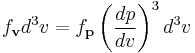
and using p = mv we get
![f_\mathbf{v} (v_x, v_y, v_z) =
\left(\frac{m}{2 \pi kT} \right)^{3/2}
\exp \left[-
\frac{m(v_x^2 %2B v_y^2 %2B v_z^2)}{2kT}
\right],
\qquad\qquad](/2012-wikipedia_en_all_nopic_01_2012/I/85cf0ae8c15fbc5d914645b864430751.png)
which is the Maxwell–Boltzmann velocity distribution. The probability of finding a particle with velocity in the infinitesimal element [dvx, dvy, dvz] about velocity v = [vx, vy, vz] is
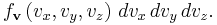
Like the momentum, this distribution is seen to be the product of three independent normally distributed variables  ,
,  , and
, and  , but with variance
  . It can also be seen that the Maxwell–Boltzmann velocity distribution for the vector velocity [vx, vy, vz] is the product of the distributions for each of the three directions:

where the distribution for a single direction is
![f_v (v_i) =
\sqrt{\frac{m}{2 \pi kT}}
\exp \left[
\frac{-mv_i^2}{2kT}
\right].
\qquad\qquad](/2012-wikipedia_en_all_nopic_01_2012/I/295ead2949493bff9984603c3e07cd27.png)
Each component of the velocity vector has a normal distribution with mean 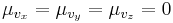 and standard deviation
 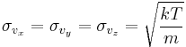 , so the vector has a 3-dimensional normal distribution, also called a "multinormal" distribution, with mean
  and standard deviation
 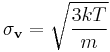 .
.
Distribution for the speed
Usually, we are more interested in the speeds of molecules rather than their component velocities. The Maxwell–Boltzmann distribution for the speed follows immediately from the distribution of the velocity vector, above. Note that the speed is
and the increment of volume is
where  and
and  are the "course" (azimuth of the velocity vector) and "path angle" (elevation angle of the velocity vector). Integration of the normal probability density function of the velocity, above, over the course (from 0 to
  ) and path angle (from 0 to
  ), with substitution of the speed for the sum of the squares of the vector components, yields the probability density function
for the speed. This equation is simply the Maxwell distribution with distribution parameter  .
.
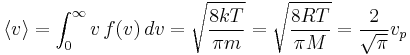
We are often more interested in quantities such as the average speed of the particles rather than the actual distribution. The mean speed, most probable speed (mode), and root-mean-square can be obtained from properties of the Maxwell distribution.
Distribution for relative speed
Relative speed is defined as  , where
 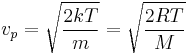 is the most probable speed. The distribution of relative speeds allows comparison of dissimilar gasses, independent of temperature and molecular weight.
Typical speeds
Although the above equation gives the distribution for the speed or, in other words, the fraction of time the molecule has a particular speed, we are often more interested in quantities such as the average speed rather than the whole distribution.
The most probable speed, vp, is the speed most likely to be possessed by any molecule (of the same mass m) in the system and corresponds to the maximum value or mode of f(v). To find it, we calculate df/dv, set it to zero and solve for v:

which yields:
Where R is the gas constant and M = NA m is the molar mass of the substance.
For diatomic nitrogen (N2, the primary component of air) at room temperature (300 K), this gives  m/s
m/s
The mean speed is the mathematical average of the speed distribution
The root mean square speed, vrms is the square root of the average squared speed:
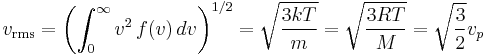
The typical speeds are related as follows:

Distribution for relativistic speeds
As the gas becomes hotter and kT approaches or exceeds mc2, the probability distribution for 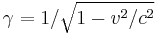 in this relativistic Maxwellian gas is given by the Maxwell–Juttner distribution[2]:
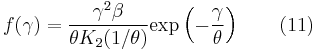
where 
 and
and  is the modified Bessel function of the second kind.
Alternatively, this can be written in terms of the momentum as
where  . The Maxwell–Juttner equation is covariant, but not manifestly so, and the temperature of the gas does not vary with the gross speed of the gas.[3]
See also
- Maxwell–Boltzmann statistics
- Boltzmann distribution
- Maxwell speed distribution
- Boltzmann factor
- Rayleigh distribution
- Ideal gas law
- James Clerk Maxwell
- Ludwig Eduard Boltzmann
- Kinetic theory
References
- ^ Laurendeau, Normand M. (2005). Statistical thermodynamics: fundamentals and applications. Cambridge University Press. p. 434. ISBN 0-521-84635-8. http://books.google.com/books?id=QF6iMewh4KMC., Appendix N, page 434
- ^ Synge, J.L (1957). The Relativistic Gas. Series in physics. North-Holland. LCCN 57-003567.
- ^ Chacon-Acosta, Guillermo; Dagdug, Leonardo; Morales-Tecotl, Hugo A. (2009). "On the Manifestly Covariant Juttner Distribution and Equipartition Theorem". arXiv:0910.1625v1. http://arxiv.org/abs/0910.1625. Retrieved 2011-10-22.
External links
- "The Maxwell Speed Distribution" from The Wolfram Demonstrations Project at Mathworld
\